
经典卷积神经网络 LeNet
Published:
本文介绍经典卷积神经网络 LeNet 的结构,说明卷积层、池化层与全连接层如何组成图像分类模型,并给出在 Fashion-MNIST 上训练和评估 LeNet 的代码。
🎦 本节课程视频地址 👇
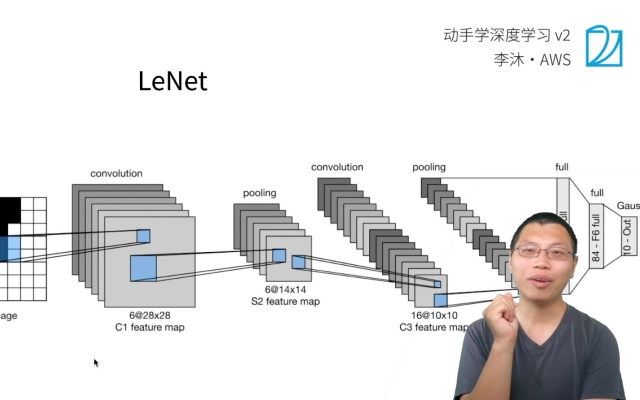
LeNet
之前我们将softmax 回归模型和多层感知机模型应用于 Fashion-MNIST 数据集中的服装图片。 为了能够应用 softmax 回归和多层感知机,我们首先将每个大小为 \((28 \times 28)\) 的图像展平为一个 784 维的固定长度的一维向量,然后用全连接层对其进行处理。 而现在,我们已经掌握了卷积层的处理方法,我们可以在图像中保留空间结构。 同时,用卷积层代替全连接层的另一个好处是:模型更简洁、所需的参数更少。
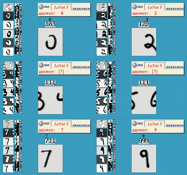
在本节中,我们将介绍LeNet,它是最早发布的卷积神经网络之一,因其在计算机视觉任务中的高效性能而受到广泛关注。 这个模型是由 AT&T 贝尔实验室的研究员 Yann LeCun 在 1989 年提出的(并以其命名),目的是识别图像 LeCun et al., 1998[1]中的手写数字。 当时,Yann LeCun 发表了第一篇通过反向传播成功训练卷积神经网络的研究,这项工作代表了十多年来神经网络研究开发的成果。
当时,LeNet 取得了与支持向量机(SVM,support vector machines)性能相媲美的成果,成为监督学习的主流方法。 LeNet 被广泛用于自动取款机(ATM)机中,帮助识别处理支票的数字。 时至今日,一些自动取款机仍在运行 Yann LeCun 和他的同事 Leon Bottou 在上世纪 90 年代写的代码呢!
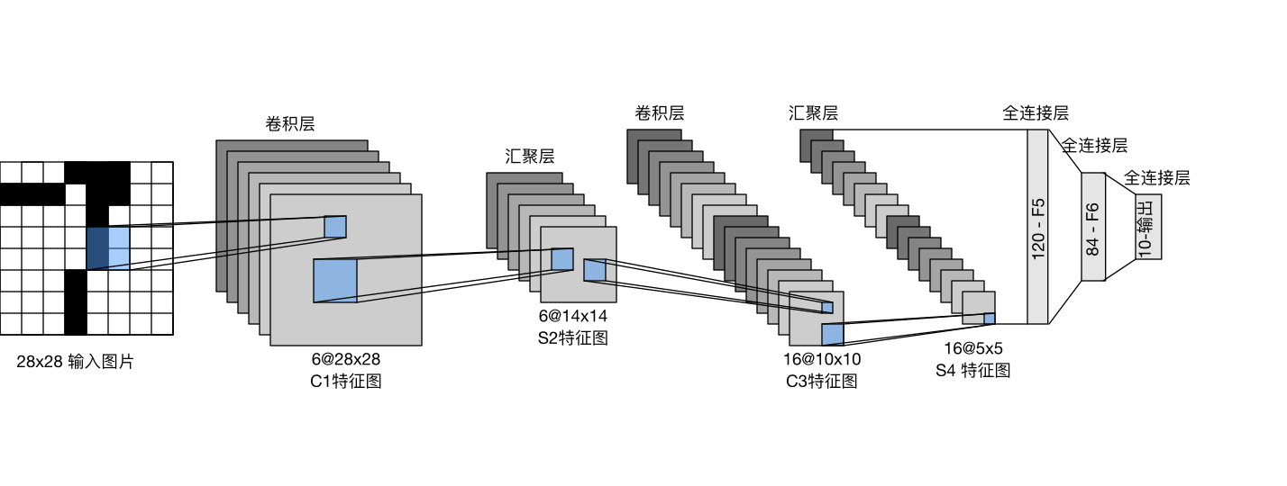
每个卷积块中的基本单元是一个卷积层、一个sigmoid 激活函数和平均汇聚层。请注意,虽然 ReLU 和最大汇聚层更有效,但它们在 20 世纪 90 年代还没有出现。每个卷积层使用\((5\times 5)\)卷积核和一个 sigmoid 激活函数。这些层将输入映射到多个二维特征输出,通常同时增加通道的数量。第一卷积层有 6 个输出通道,而第二个卷积层有 16 个输出通道。每个\((2\times2)\)池操作(步骤 2)通过空间下采样将维数减少 4 倍。卷积的输出形状由批量大小、通道数、高度、宽度决定。
为了将卷积块的输出传递给稠密块,我们必须在小批量中展平每个样本。换言之,我们将这个四维输入转换成全连接层所期望的二维输入。这里的二维表示的第一个维度是索引小批量中的样本,第二个维度是给出每个样本的平面向量表示。LeNet 的稠密块有三个全连接层,分别有 120、84 和 10 个输出。因为我们在执行分类任务,所以输出层的 10 维对应于最后输出结果的数量。
总结
- 是早期成功的神经网络
- 先使用卷积层来学习图片的空间信息
- 然后使用全连接层来转换到类别空间。
代码实现
- 定义网络
import torch
from torch import nn
from d2l import torch as d2l

class Reshape(torch.nn.Module):
    def forward(self, x):
        return x.view(-1, 1, 28, 28)
        #Returns a new tensor with the same data as the self tensor
        #but of a different shape
        #批量不变,通道唯一,

net = torch.nn.Sequential(
    Reshape(), nn.Conv2d(1, 6, kernel_size=5, padding=2), nn.Sigmoid(),
    nn.AvgPool2d(kernel_size=2, stride=2),
    nn.Conv2d(6, 16, kernel_size=5), nn.Sigmoid(),
    nn.AvgPool2d(kernel_size=2, stride=2),
    # nn.Flatten()默认从第1维到最后一维展平,保留第0维批量维
    nn.Flatten(),
    nn.Linear(16 * 5 * 5, 120), nn.Sigmoid(),
    nn.Linear(120, 84), nn.Sigmoid(),
    nn.Linear(84, 10))
- 测试
X = torch.rand(size=(1, 1, 28, 28), dtype=torch.float32)
for layer in net:
    X = layer(X)
    print(layer.__class__.__name__, 'output shape: \t', X.shape)
    #调用layer的名字
- 训练
batch_size = 256
train_iter, test_iter = d2l.load_data_fashion_mnist(batch_size=batch_size)

def evaluate_accuracy_gpu(net, data_iter, device=None):
    if isinstance(net, torch.nn.Module):
        net.eval()
        if not device:
            device = next(iter(net.parameters())).device
            #查看存储设备
        metric = d2l.Accumulator(2)
        for X, y in data_iter:
            if isinstance(X, list):
                X = [x.to(device) for x in X]
            else:
                X = X.to(device)
            y = y.to(device)
            metric.add(d2l.accuracy(net(X), y), y.numel())
        return metric[0] / metric[1]
- 训练函数
def train_ch6(net, train_iter, test_iter, num_epochs, lr, device):
    def init_weights(m):
        if type(m) == nn.Linear or type(m) == nn.Conv2d:
            nn.init.xavier_uniform_(m.weight)
    net.apply(init_weights)
    print('training on', device)
    net.to(device)
    optimizer = torch.optim.SGD(net.parameters(), lr=lr)
    loss = nn.CrossEntropyLoss()
    #默认取平均损失
    animator = d2l.Animator(xlabel='epoch', xlim=[1, num_epochs],
                           legend=['train loss', 'train acc', 'test acc'])
    timer, num_batches = d2l.Timer(), len(train_iter)
    for epoch in range(num_epochs):
        metric = d2l.Accumulator(3)
        # metric.data=[0.,0.,0.]
        net.train()
        for i, (X, y) in enumerate(train_iter):
            # X.shape=(256,1,28,28)
            timer.start()
            optimizer.zero_grad()
            X, y = X.to(device), y.to(device)
            y_hat = net(X)
            l = loss(y_hat, y)
            l.backward()
            optimizer.step()
            metric.add(l * X.shape[0], d2l.accuracy(y_hat, y), X.shape[0])
            #返回三个标量,l*256,accuracy,256

            timer.stop()
            train_l = metric[0] / metric[2]
            #平均损失
            train_acc = metric[1] / metric[2]
            #正确率
            if (i + 1) % (num_batches // 5) == 0 or i == num_batches - 1:
                animator.add(epoch + (i + 1) / num_batches,
                             (train_l, train_acc, None))
        test_acc = evaluate_accuracy_gpu(net, test_iter)
        animator.add(epoch + 1, (None, None, test_acc))
    print(f'loss {train_l:.3f}, train acc {train_acc:.3f}, '
          f'test acc {test_acc:.3f}')
    print(f'{metric[2] * num_epochs / timer.sum():.1f} examples/sec '
          f'on {str(device)}')
lr, num_epochs = 0.9, 10
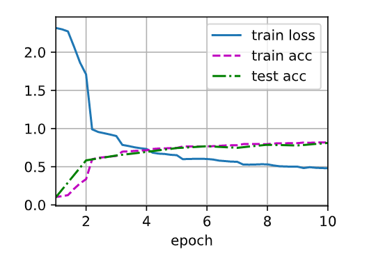
train_ch6(net, train_iter, test_iter, num_epochs, lr, d2l.try_gpu())
参考资料
[2]cnn explianer:一个卷积神经网络可视化 Demo
Q&A🤓
Q:max pooling 和 average pooling 哪个用的更多?
🙋♂️:二者差别不大(可能在具体问题有细微差别),一般来说 max pooling 用的更多,因为 max pooling 得到的数值更大,相对梯度比 average 也个更大,更好训练。