
D2L-40 序列模型
Published:
本文介绍具有时间结构的序列数据,讨论自回归模型、隐变量自回归模型和马尔可夫假设,并通过时间序列预测代码比较不同预测方式。
🎦 本节课程视频地址 👇

序列模型
- 实际中很多数据是有时序结构的
- 如电影的评分
- 音乐、语言、文本和视频都是连续的
- 股票的价格
- 人与人之间的互动
统计工具
- 在时间 \(t\) 观察到 \(x_t\),那么得到 \(T\) 个不独立的随机变量 \((x_1,...,x_T)~p(\bf x)\)
- 使用条件概率展开(贝叶斯公式) \(p(a,b)=p(a)p(b\vert a)=p(b)p(a\vert b)\)
推广到这一系列事件同时发生的概率,换言之,前 \(T-1\) 个事件已经发生的条件下,第 \(T\) 个事件发生的概率:
正向:
\[p({\bf x})=p(x_1)\cdot p(x_2\vert x_1)\cdot p(x_3\vert x_1,x_2)\cdot ...\cdot p(x_T\vert x_1,...,x_{T-1})\]反向:
\[p({\bf x})=p(x_T)\cdot p(x_{T-1}\vert x_T)\cdot p(x_{T-2}\vert x_{T-1},x_T)\cdot ...\cdot p(x_1\vert x_{T-1},...,x_2)\]反向从未来推广到过去,并不完全有物理意义
对条件概率建模:
\[p(x_t\vert x_1,...,x_{t-1})=p(x_t\vert f(x_1,...,x_{t-1}))\]对见过的数据建模,也称自回归模型(Autoregressive Model)。
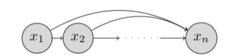
马尔科夫假设
假设当前数据只跟 \(\tau\) 个过去数据点相关
\[p(x_t\vert x_1,...,x_{t-1})=p(x_t\vert x_{t-\tau},...,x_{t-1})=p(x_t\vert f(x_{t-\tau},...,x_{t-1}))\]潜变量模型
引入潜变量 \(h_t\) 来表示过去信息 \(h_t=f(x_1,...,x_{t-1})\)
- 这样 \(x_t=p(x_t\vert h_t)\)
总结
- 在时序模型中,当前数据跟之前观察到的数据相关
- 自回归模型使用自身过去数据来预测未来
- 马尔可夫模型假设当前只跟最近少数数据相关
- 潜变量模型使用潜变量来概括历史信息
代码模拟马尔可夫算法
创建数据集
%matplotlib inline
import torch
from torch import nn
from d2l import torch as d2l

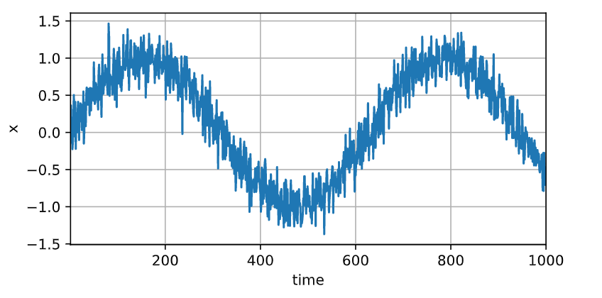
T = 1000  # 总共产生1000个点
time = torch.arange(1, T + 1, dtype=torch.float32)
x = torch.sin(0.01 * time) + torch.normal(0, 0.2, (T,))
#torch.normal(mean, std, size)
d2l.plot(time, [x], 'time', 'x', xlim=[1, 1000], figsize=(6, 3))
tau = 4
features = torch.zeros((T - tau, tau))
#(996, 4)全零
for i in range(tau):
    features[:, i] = x[i: T - tau + i]
    #对每行的第i列赋值,996行
    #按顺序把每四个点作为一个样本
    #每次向前一个点
labels = x[tau:].reshape((-1, 1))
#预测点实值x(4:1000),转化为列向量
batch_size, n_train = 16, 600
#把前600个样本用于训练
train_iter = d2l.load_array((features[:n_train], labels[:n_train]),
                            batch_size, is_train=True) #x[599:603]
#Construct a PyTorch data iterator.
网络和训练
#定义MLP网络
def init_weights(m):
    if type(m) == nn.Linear:
        nn.init.xavier_uniform_(m.weight)

def get_net():
    net = nn.Sequential(nn.Linear(4, 10),
                        nn.ReLU(),
                        nn.Linear(10, 1))
    net.apply(init_weights)
    return net

loss = nn.MSELoss(reduction='none')

def train(net, train_iter, loss, epochs, lr):
    trainer = torch.optim.Adam(net.parameters(), lr)
    for epoch in range(epochs):
        for X, y in train_iter:
            trainer.zero_grad()
            l = loss(net(X), y)
            l.sum().backward()
            trainer.step()
        print(f'epoch {epoch + 1}, '
              f'loss: {d2l.evaluate_loss(net, train_iter, loss):f}')

net = get_net()
train(net, train_iter, loss, 5, 0.01)
#在这里已经训练好了网络的权重,所以在后面直接调用就可以了
预测
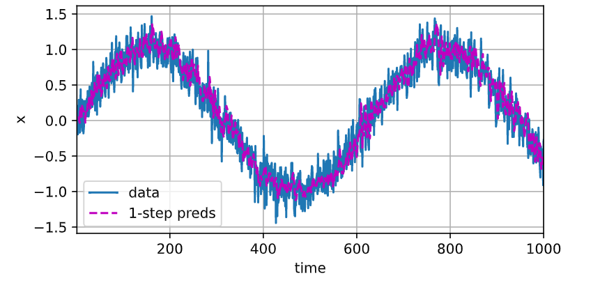
onestep_preds = net(features)
#对整个样本进行预测
d2l.plot([time, time[tau:]],
         [x.detach().numpy(), onestep_preds.detach().numpy()], 'time',
         'x', legend=['data', '1-step preds'], xlim=[1, 1000],
         figsize=(6, 3))
#分别对于实际和预测绘图
multistep_preds = torch.zeros(T)
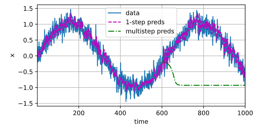
multistep_preds[: n_train + tau] = x[: n_train + tau]
#(0:604)
for i in range(n_train + tau, T):
    #(604,1000)
    multistep_preds[i] = net(
        multistep_preds[i - tau:i].reshape((1, -1)))
    #[600,604]用于预测604并赋值
    #实际上前599个并没有起作用

#从前603个预测后面的396个
#所以很离谱

d2l.plot([time, time[tau:], time[n_train + tau:]],
         [x.detach().numpy(), onestep_preds.detach().numpy(),
          multistep_preds[n_train + tau:].detach().numpy()], 'time',
         'x', legend=['data', '1-step preds', 'multistep preds'],
         xlim=[1, 1000], figsize=(6, 3))
max_steps = 64

features = torch.zeros((T - tau - max_steps + 1, tau + max_steps))
#(993, tau+max_steps)
for i in range(tau):
    features[:, i] = x[i: i + T - tau - max_steps + 1]
    #给前tau个赋值

for i in range(tau, tau + max_steps):
    features[:, i] = net(features[:, i - tau:i]).reshape(-1)
    #预测后max_steps个

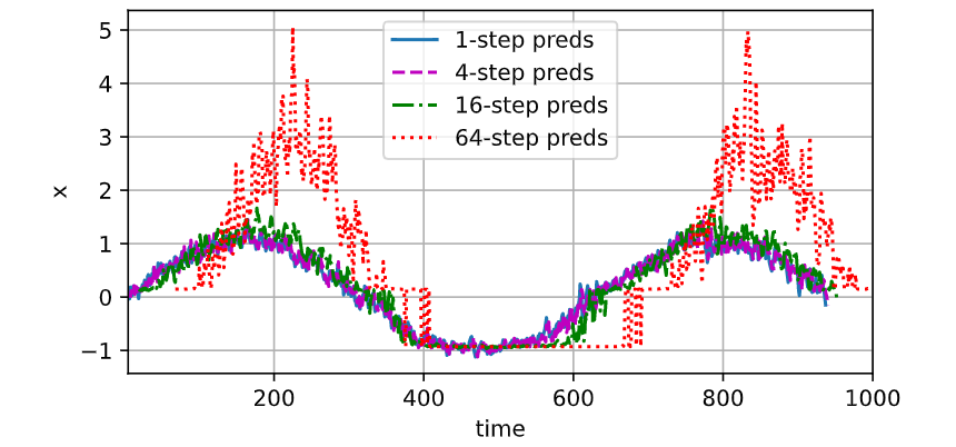
steps = (1, 4, 16, 64)
d2l.plot([time[tau + i - 1: T - max_steps + i] for i in steps],
         [features[:, (tau + i - 1)].detach().numpy() for i in steps], 'time', 'x',
         legend=[f'{i}-step preds' for i in steps], xlim=[5, 1000],
         figsize=(6, 3))
    # steps = 1
    # time[4: 937]
    # features[:, 4] 画每行第五个元素
    # steps = 4
    # time[7: 937]
    # features[:, 7] 画每行第八个元素,或者说5-8个元素是预测出来的,只选择第8个

#实际上这个算法的底层逻辑都是用前4个预测第5个,然后依次类推,直到max_step处
#画图是为了把第step处的预测表示出来
#也就是表示出预测到不同位置的拟合程度
一点感悟
逻辑比代码本身更重要。
体现在代码里,就是通过简单的切片代替复杂的循环,实现想要达到的效果,这非常了不起。