
D2L-25 含并行连接的网络 GoogLeNet
Published:
本文介绍含并行连接的 GoogLeNet,分析 Inception 块如何组合不同尺寸的卷积与池化操作,并通过代码展示多分支网络的组织与训练方式。
🎦 本节课程视频地址 👇
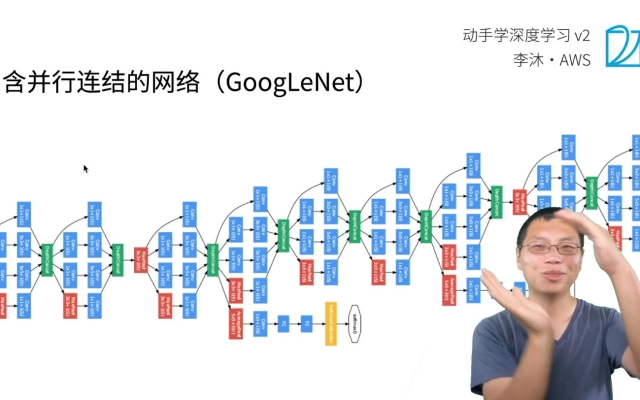
问题的引出
在 2014 年的 ImageNet 图像识别挑战赛中,一个名叫 GoogLeNet [Szegedy et al., 2015]的网络架构大放异彩。 GoogLeNet 吸收了 NiN 中串联网络的思想,并在此基础上做了改进。 这篇论文的一个重点是解决了什么样大小的卷积核最合适的问题。 毕竟,以前流行的网络使用小到 1×1 ,大到 11×11 的卷积核。 该文的一个观点是,有时使用不同大小的卷积核组合是有利的。
Inception 块
在 GoogLeNet 中,基本的卷积块被称为Inception 块(Inception block)。这很可能得名于电影《盗梦空间》(Inception),因为电影中的一句话“我们需要走得更深”(“We need to go deeper”)。

Inception 块使用用 4 个路径从不同层面抽取信息,然后在输出通道维合并。
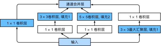
- 输出和输入等高宽,将 4 条路径的结果按通道合并
- 1x1 卷积层:进行通道融合,降低通道数来控制模型复杂度
- 非 1x1 的卷积层、MaxPooling:提取空间特性,增加鲁棒性
- 每条路径的通道数可能不一样
Inception 的优势
跟单 3x3 或 5x5 卷积层相比,输出相同通道数,Inception 块只需要更少的参数个数和计算复杂度.
| #parameters | FLOPS | |
|---|---|---|
| Inception | 0.16M | 128M |
| 3x3 Conv | 0.44M | 346M |
| 5x5 Conv | 1.22M | 963M |
FLOPS,Floating-point Operations Per Second
GoogLeNet
包含 5 Stages, 9 Inception 块
- 架构图
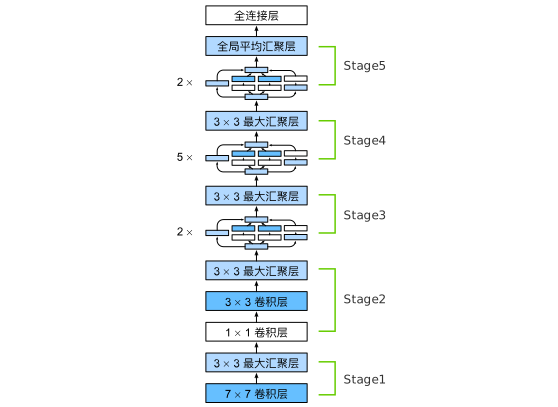
- 各层信息
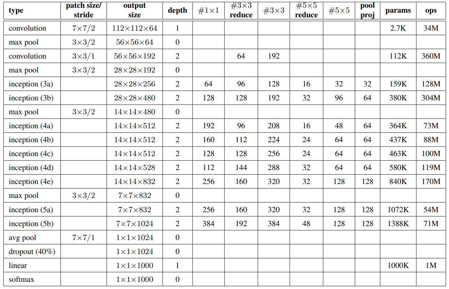
Inception 变种
- Inception-BN(V2):使用了 batch normalization
- Inception-V3:修改了 Inception(包含诡异的 1x3、3x1、1x7、7x1Conv)
- Inception-V4:使用残差连接
总结
- Inception 块使用 4 条有不同超参数的卷积层和池化层的通路来抽取不同的信息
- 一个主要优点是模型参数小,计算复杂度低
- GooLeNet 用了 9 个 Inception 块,是第一个达到上百层的网络
- 后续有一系列改进变种
代码实现
- 实现 Inception 块
import torch
from torch import nn
from torch.nn import functional as F
from d2l import torch as d2l

class Inception(nn.Module):
    # c1~c4表示四条路径的通道数
    def __init__(self, in_channels, c1, c2, c3, c4, **kwargs):
        super(Inception, self).__init__(**kwargs) #继承父类属性

        #pass1 1x1conv
        self.p1_1 = nn.Conv2d(in_channels, c1, kernel_size=1) #Conv2d, default_stride=1, default_padding=0
        #pass2 1x1+3x3conv
        self.p2_1 = nn.Conv2d(in_channels, c2[0], kernel_size=1)
        self.p2_2 = nn.Conv2d(c2[0], c2[1], kernel_size=3, padding=1)
        #pass3 1x1+5x5conv
        self.p3_1 = nn.Conv2d(in_channels, c3[0], kernel_size=1)
        self.p3_2 = nn.Conv2d(c3[0], c3[1], kernel_size=5, padding=2)
        #pass4 3x3MaxPool+1x1conv
        self.p4_1 = nn.MaxPool2d(kernel_size=3, stride=1, padding=1)
        self.p4_2 = nn.Conv2d(in_channels, c4, kernel_size=1)

    def forward(self, x):
        p1 = F.relu(self.p1_1(x))
        p2 = F.relu(self.p2_2(F.relu(self.p2_1(x))))
        p3 = F.relu(self.p3_2(F.relu(self.p3_1(x))))
        p4 = F.relu(self.p4_2(self.p4_1(x)))
        # .cat(dim=1)在通道维dim=1合并结果
        return torch.cat((p1, p2, p3, p4), dim=1)
- 定义 Stage1 结构:使用 64 个通道、 7×7 卷积层
b1 = nn.Sequential(nn.Conv2d(1, 64, kernel_size=7, stride=2, padding=3),nn.ReLU(),
                   nn.MaxPool2d(kernel_size=3, stride=2, padding=1))
- 定义 Stage2 结构:第一个卷积层是 64 个通道、 1×1 卷积层;第二个卷积层使用将通道数量增加三倍的 3×3 卷积层
b2 = nn.Sequential(nn.Conv2d(64, 64, kernel_size=1),nn.ReLU(),
                   nn.Conv2d(64, 192, kernel_size=3, padding=1),nn.ReLU(),
                   nn.MaxPool2d(kernel_size=3, stride=2, padding=1))
- 定义 Stage3 结构:第一个 Inception 块的输出通道数为 64+128+32+32=256。第二个 Inception 块的输出通道数增加到 128+192+96+64=480
b3 = nn.Sequential(Inception(192, 64, (96, 128), (16, 32), 32),
                   Inception(256, 128, (128, 192), (32, 96), 64),
                   nn.MaxPool2d(kernel_size=3, stride=2, padding=1))
- 定义 Stage4 结构:串联 5 个 Inception 块
b4 = nn.Sequential(Inception(480, 192, (96, 208), (16, 48), 64),
                   Inception(512, 160, (112, 224), (24, 64), 64),
                   Inception(512, 128, (128, 256), (24, 64), 64),
                   Inception(512, 112, (144, 288), (32, 64), 64),
                   Inception(528, 256, (160, 320), (32, 128), 128),
                   nn.MaxPool2d(kernel_size=3, stride=2, padding=1))
- 定义 Stage5 结构:两个 Inception 块后面紧跟输出层
b5 = nn.Sequential(Inception(832, 256, (160, 320), (32, 128), 128),
                   Inception(832, 384, (192, 384), (48, 128), 128),
                   nn.AdaptiveAvgPool2d((1,1)),
                   nn.Flatten())

net = nn.Sequential(b1, b2, b3, b4, b5, nn.Linear(1024, 10))
- 测试各层输出
X = torch.rand(size=(1, 1, 96, 96))
for layer in net:
    X = layer(X)
    print(layer.__class__.__name__,'output shape:\t', X.shape)

# Out:
# Sequential output shape:     torch.Size([1, 64, 24, 24])
# Sequential output shape:     torch.Size([1, 192, 12, 12])
# Sequential output shape:     torch.Size([1, 480, 6, 6])
# Sequential output shape:     torch.Size([1, 832, 3, 3])
# Sequential output shape:     torch.Size([1, 1024])
# Linear output shape:         torch.Size([1, 10])
- 训练
lr, num_epochs, batch_size = 0.1, 10, 128
train_iter, test_iter = d2l.load_data_fashion_mnist(batch_size, resize=96)
d2l.train_ch6(net, train_iter, test_iter, num_epochs, lr, d2l.try_gpu())

# Out:
# loss 0.244, train acc 0.908, test acc 0.896
# 3490.2 examples/sec on cuda:0
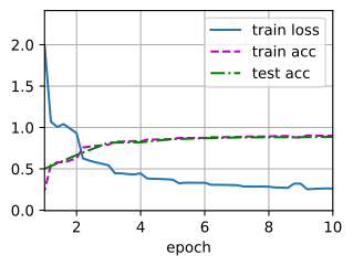
配图说明:部分旧版图片链接已失效,现采用教材对应章节中的 PyTorch 示例图;图中数值可能与笔记保留的历史运行输出略有不同。